Excel Practice

Negative Numbers in Excel

Typing Negative Numbers

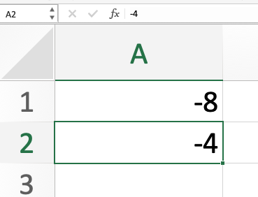
Negative numbers are typed into Excel by using a hyphen - symbol and the number.

Example: negative 3 is typed “-3” without the quotation marks

Cell Formatting

In this course we will always show negative numbers as black numbers with a negative symbol in front of them, however, there are other ways to display negative numbers in Excel. Some of these other notations are used in accounting, bookkeeping, and finance.

Cells can be formatted so that negative numbers display differently.

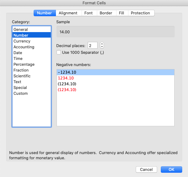
Go to the “Format Cell” window by right clicking on a cell you want to format.

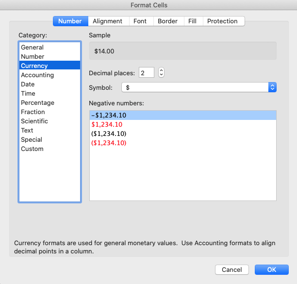
Under the “Number” tab select the “Number” or “Currency” category.

In the Number category you will see 4 options for negative numbers:

-1234.10 = This option keeps negative numbers black with a negative symbol in front.
1234.10 = This option turns negative numbers typed into these cells red without a negative symbol.
(1234.10) = This option keeps the negative number black but displays them with parentheses around them. This notation is often used in accounting and bookkeeping.
(1234.10) = This option turns negative numbers red and displays them with parentheses around them.

In the Currency category, the options are the same except they are also displayed with a currency symbol.

For this class and in general, we recommend using the standard - hyphen to show a number is negative.

Arithmetic with Negative Numbers

The arithmetic on negative numbers is the same as on positive numbers in Excel.

You can reference cells with negative numbers just as you would positive numbers. You can also write equations with negative numbers.

Example: Type “-3*-5+-1” into a cell. Type enter. You should see the number 14 appear in the cell because (-3)(-5)+(-1)=15+(-1)=14

and 15+-1=14.

Note: You may want to use parentheses in examples like this to make them more readable. Excel will follow the order of operation.