Excel Practice
Percentages in Excel
Video Source (05:19 mins) | Transcript
There are many ways to format a cell as a percentage in Excel. This lesson goes over the following 4 ways.
This lesson also teaches how to format several cells at once.
Number and % symbol
Typing a number into the cell.
At the end of the number type the % symbol.
Type enter.
This will automatically tell Excel that the number you typed is a percentage and it will format the cell as a percentage cell so that any number you put in the cell will show up with a % symbol.
Format Cell
Right click on the cell you want to display as a percentage.
A menu will appear. Click on the “Format Cell” item on the list.
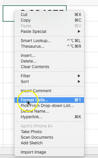
This will bring up the Format Cell window.
Under the Numbers tab you will see a category list of all the number formats you can assign to a cell. Click on the Percentage category.
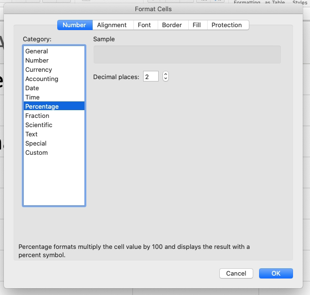
Notice that you can change the number of decimal places displayed in the Decimal places box. You can use this box to adjust the decimal places no matter what approach you originally used to format the cell as a percentage.
Number Format Menu
In the Home Toolbar you will find the number format menu box. The default in the box says “General.”

Click on the arrow to the right of the box to bring down the other options. Select the “Percentage” item on the list.
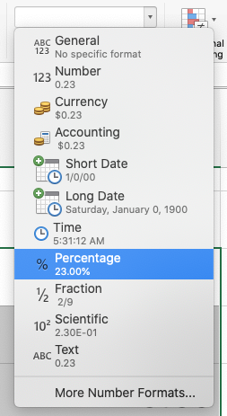
This will automatically format the cell as a percentage with two places after the decimal point. You can adjust the places after the decimal point using the format cell technique explained above.
% Style Button
Select the cell you want to format by clicking within it.
Click on the % style button in the Home Toolbar. It is a button with a % symbol in it.
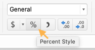
This will format the cell to display as a percentage.
Format Several Cells At Once
Highlight all the cells you want to format as a percentage.
Example image:
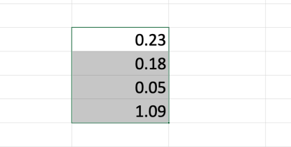
Once the cells are selected, use either the Format Cell, Number Format Menu, or % Style Button technique to format the cells as percentages.