Excel Practice
Subtraction using Excel
You can watch the video or just read the text below. Both will give you the same information.
The following topics are covered in this lesson.
- Using the hyphen symbol for subtraction
- Referencing Cells and using the hyphen symbol for subtraction
- Subtraction = Adding negative numbers
Video Source (04:28 mins) | Transcript
Using the hyphen symbol for subtraction
Referencing Cells and using the hyphen symbol for subtraction
Subtraction = Adding negative numbers
Using the hyphen symbol
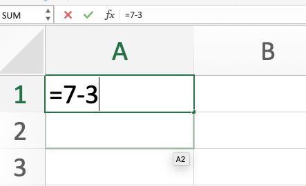
If you want to use Excel as a calculator, first click on the cell of your choice. Type “=” (without the quote marks) and then type the numbers separated by a hyphen “-”.
Example: Find the answer to 7-3 in a cell.
Answer: In Excel type “=7-3” (without the quotation marks). When you click enter, the number 4 will appear in the cell.
Click “enter”.
The number 4 will appear in the cell because 7-3=4
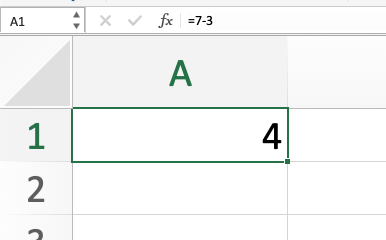
Notice that the equation “=7-3” is still seen in the formula bar at the top of Excel
Why start with an equal sign?
You are telling Excel that you want the cell you have clicked on to be equal to the equation after the equal sign.
Referencing Cells and using the hyphen symbol for subtraction
You can subtract the values in different cells by referencing them just as you do with addition or any other mathematical operation.
Example:
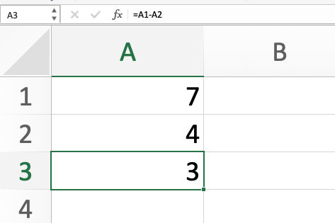
The number 7 is in A1 and the number 4 is in A2.
Subtract 7- 4 in another cell using the cell references for A1 and A2.
Answer: In cell A3 type “=A1-A2” (without the quotation marks)
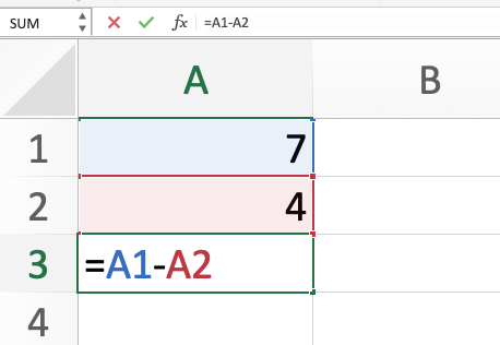
Click “enter”.
The number 3 appears in cell A3 because 7-4=3.
The advantage of doing this is that the numbers in cells A1 and A2 can change and the value in A3 will automatically calculate the new equation.
Example:
Change A1 to 8.
Notice that the value in A3 automatically changes to 4 because 8-4=4
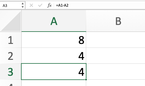
Both of the numbers in A1 and A2 can change because we are using references for both of them.
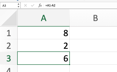
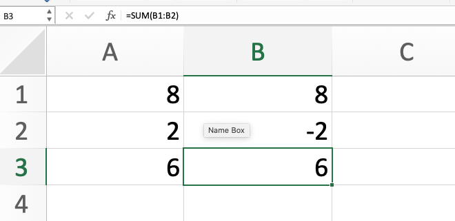
Example: Change A2 to the number 6. Notice that A3 automatically changes to 6 since 8-2=6.
Subtraction = Adding Negative Numbers
Subtraction is actually the same as adding a negative number. This is particularly handy in Excel.
Example: Calculate 8-2 but using the concept of adding a negative number and using the SUM function.
In B1 type 8
In B2 type -2
In B3 use the sum function to add B1 and B2 together by typing into it “=sum(B1:B2)”
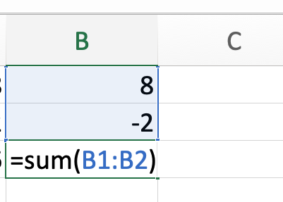
Click “enter”.
Notice that the number 6 appears in cell B3. This is the same answer we calculated in cell A3 in our previous example using subtraction and referencing cells.
Making the 2 a negative number and then adding the cells together is the same as subtracting.
This technique is particularly helpful when adding negative and positive numbers together in Excel.
Example: Imagine a column of numbers in Excel, some positive and some negative.
C1=4
C2=-7
C3=-3
C4=10
C5=-2
C6=-1.
We could add them all together individually, or we could use the sum function by typing in “=sum(C1:C6)”.
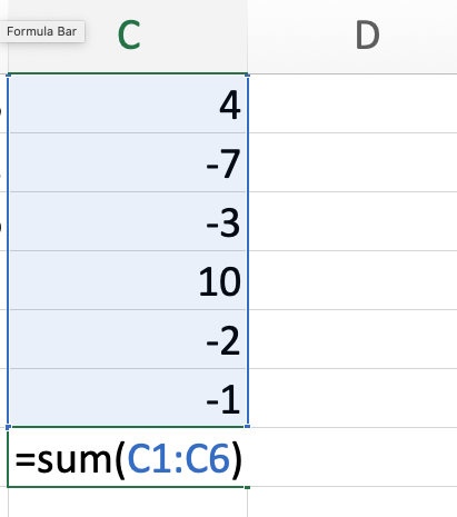
Click “enter”.
The number 1 appears in our new cell.
Subtracting a Negative Number
When subtracting a negative number it is helpful to use parentheses around the negative number to more easily see both the subtraction symbol and the negative symbol.
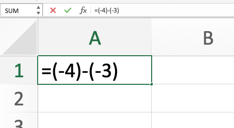
Example: Calculate (-4) - (-3) using Excel.
Answer: Click on a cell. Type “=-4-(-3)” (without quotation marks)
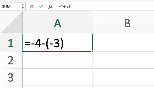
When you click “enter”, the number -1 will appear in the cell because (-4)-(-3)=-1.
In this case the parentheses are only there to help us see what is happening. Excel can calculate this without the parentheses as well.
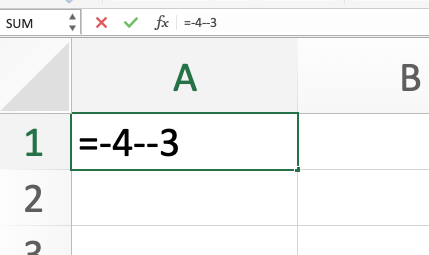
Notice how it is hard to see the negative next to the subtraction symbol since they are the same symbol.
We could also put parentheses around the -4 as well.