Pandas Tutorial
Overview
This tutorial walks through the fundamentals of the Pandas data science library.
Preparation
For this tutorial, you will need the Pandas library for data manipulation as well as the Seaborn library for visualization. Then you will need to download the data.
Install the Libraries
There are two primary ways to install these libraries. The first is to use a package manager that is included in an IDE such as Thonny. The second is to use a command line install tool, like PIP.
If you are using an IDE with a package manager, such as Thonny, select Tools -> Manage Packages. Search for pandas and install it. Then, search for seaborn and install it as well.
If you are installing these libraries from the command line, you can type pip install pandas and pip install seaborn . To install them.
Instructor Tip
If you are trying to use the pip installer, you will likely need to have administrative privileges by running "sudo pip install pandas" on Mac/Linux or, if you are using Windows, you can right click the Command Line utility and select "Run as Administrator" rather than running it directly.
If you are trying to use the pip installer and encounter an error message similar to a "command not found" it is likely that the directory containing this utility is not in your path (the place where your computer looks for applications to run). You may need to find the pip utility yourself and then add the folder that contains it, to the path.
Downloading the Dataset
This tutorial uses a dataset of NBA basketball statistics that can be downloaded here. This dataset was originally obtained from opensourcesports.com and can also be found at Kaggle. It did not come with an explicit license, but based on other datasets from Open Source Sports, we treat it as follows: This database is copyright 1996-2015 by Sean Lahman. This work is licensed under a Creative Commons Attribution-ShareAlike 3.0 Unported License. For details see: http://creativecommons.org/licenses/by-sa/3.0/
The dataset is contained in several files contained in a ZIP file. You should download and extract the ZIP file, then you can copy the .csv (comma separated values) files contained in the ZIP file into another directory to work with. It is most convenient to put these .csv files in the same directory as your .py python script.
The two primary files we will use from this dataset are:
basketball_players.csv - This file contains the stats for each player for a given season.
basketball_master.csv - This file contains additional information about the players, such as biographical information, etc.
Loading the libraries and data files in Python
The first step is to load the libraries.
import pandas as pd # Our data manipulation library
import seaborn as sns # Used for graphing/plotting
import matplotlib.pyplot as plt # If we need any low level methods
import os # Used to change the directory to the right place
The next step is to load the data itself.
# This line isn't necessary, but it makes it so the later commands (e.g., read_csv)
# are in a consistent place (You will obviously need to change this to the correct location on _your_ computer.)
# If you have put the data files and your Python script in the same folder, you
# don't need this line.
os.chdir("/Users/sburton/cs241/nbaData/")

# Load in the data
# The players data (basketball_players.csv) has the season stats
players = pd.read_csv("basketball_players.csv")
After running the above commands, I received the following message:
/Library/Frameworks/Python.framework/Versions/3.6/lib/python3.6/site-packages/IPython/core/interactiveshell.py:2705:
DtypeWarning: Columns (41) have mixed types. Specify dtype option on import or set low_memory=False.
  interactivity=interactivity, compiler=compiler, result=result)
The above error message says that some column data types could not be determined automatically, or seemed to be mixed. We can avoid this by specifying them directly, but in this case, we will ignore it, and move on to look at the data.
With the players dataset loaded, we can play with it to see different things.
players
Instructor Tip:
If you are running the commands directly in the interactive Python console, you can just type an expression or the name of the dataset variable directly and it will display the results. If you are putting it into a script, you'll need to print the results (e.g., "print(players)") rather than just typing the name of the variable.
playerID year stint tmID lgID GP GS minutes points oRebounds \
0 abramjo01 1946 1 PIT NBA 47 0 0 527 0
1 aubucch01 1946 1 DTF NBA 30 0 0 65 0
2 bakerno01 1946 1 CHS NBA 4 0 0 0 0
3 baltihe01 1946 1 STB NBA 58 0 0 138 0
4 barrjo01 1946 1 STB NBA 58 0 0 295 0
5 baumhfr01 1946 1 CLR NBA 45 0 0 631 0
6 beckemo01 1946 1 PIT NBA 17 0 0 108 0
7 beckemo01 1946 2 BOS NBA 6 0 0 13 0
8 beckemo01 1946 3 DTF NBA 20 0 0 41 0
9 beendha01 1946 1 PRO NBA 58 0 0 713 0
10 biasaha01 1946 1 TRH NBA 6 0 0 6 0
11 brighal01 1946 1 BOS NBA 58 0 0 567 0
12 brindau01 1946 1 NYK NBA 12 0 0 34 0
13 brownha01 1946 1 DTF NBA 54 0 0 264 0
14 brownle01 1946 1 CLR NBA 5 0 0 0 0
15 byrneto01 1946 1 NYK NBA 60 0 0 453 0
16 bytzumi01 1946 1 PIT NBA 60 0 0 210 0
17 callato01 1946 1 PRO NBA 13 0 0 17 0
18 calveer01 1946 1 PRO NBA 59 0 0 845 0
19 carlich01 1946 1 CHS NBA 51 0 0 256 0
20 carlsdo01 1946 1 CHS NBA 59 0 0 630 0
21 cluggbo01 1946 1 NYK NBA 54 0 0 238 0
22 connoch01 1946 1 BOS NBA 49 0 0 227 0
23 corleke01 1946 1 CLR NBA 3 0 0 0 0
24 crislha01 1946 1 BOS NBA 4 0 0 6 0
25 curear01 1946 1 PRO NBA 12 0 0 10 0
26 dallmho01 1946 1 PHW NBA 60 0 0 528 0
27 davisau01 1946 1 STB NBA 59 0 0 287 0
28 davisbi01 1946 1 CHS NBA 47 0 0 84 0
29 dehnehe01 1946 1 PRO NBA 10 0 0 14 0
... ... ... ... ... .. .. ... ... ...
23721 lacoufr01 1962 0 OAO ABL1 25 0 901 494 0
23722 millsda01 1962 0 OAO ABL1 21 0 359 155 0
23723 romanni01 1962 0 OAO ABL1 25 0 755 225 0
23724 toddro01 1962 0 OAO ABL1 24 0 733 339 0
23725 turneja02 1962 0 OAO ABL1 25 0 930 373 0
23726 vaughgo01 1962 0 OAO ABL1 22 0 350 122 0
23727 wilkibo01 1962 0 OAO ABL1 23 0 339 128 0
23728 yateswa01 1962 0 OAO ABL1 25 0 624 268 0
23729 bellwh01 1962 0 PGR ABL1 7 0 223 69 0
23730 curtich01 1962 0 PGR ABL1 22 0 666 301 0
23731 curtihe01 1962 0 PGR ABL1 20 0 596 275 0
23732 hawkico01 1962 0 PGR ABL1 16 0 668 447 0
23733 kennewa01 1962 0 PGR ABL1 5 0 91 50 0
23734 manghwa01 1962 0 PGR ABL1 22 0 529 213 0
23735 mccarjo01 1962 0 PGR ABL1 18 0 420 95 0
23736 mccoyji01 1962 0 PGR ABL1 22 0 847 350 0
23737 rolliph01 1962 0 PGR ABL1 17 0 611 221 0
23738 tyrach01 1962 0 PGR ABL1 23 0 518 212 0
23739 wiesebo01 1962 0 PGR ABL1 15 0 252 101 0
23740 alixlo01 1962 0 PHT ABL1 1 0 3 0 0
23741 blyesy01 1962 0 PHT ABL1 28 0 975 496 0
23742 chmiemo01 1962 0 PHT ABL1 20 0 528 208 0
23743 clarkbo01 1962 0 PHT ABL1 16 0 217 59 0
23744 hillcl01 1962 0 PHT ABL1 22 0 422 145 0
23745 johnsan01 1962 0 PHT ABL1 28 0 732 314 0
23746 kaisero01 1962 0 PHT ABL1 27 0 978 467 0
23747 spragbr01 1962 0 PHT ABL1 27 0 746 356 0
23748 tayloro02 1962 0 PHT ABL1 28 0 1007 355 0
23749 wellsra01 1962 0 PHT ABL1 2 0 36 4 0
23750 wrighle01 1962 0 PHT ABL1 28 0 813 195 0
... PostBlocks PostTurnovers PostPF PostfgAttempted PostfgMade \
0 ... 0 0 0 0 0
1 ... 0 0 0 0 0
2 ... 0 0 0 0 0
3 ... 0 0 3 10 2
4 ... 0 0 0 0 0
5 ... 0 0 0 0 0
6 ... 0 0 0 0 0
7 ... 0 0 0 0 0
8 ... 0 0 0 0 0
9 ... 0 0 0 0 0
10 ... 0 0 0 0 0
11 ... 0 0 0 0 0
12 ... 0 0 4 6 3
13 ... 0 0 0 0 0
14 ... 0 0 0 0 0
15 ... 0 0 2 46 11
16 ... 0 0 0 0 0
17 ... 0 0 0 0 0
18 ... 0 0 0 0 0
19 ... 0 0 33 88 20
20 ... 0 0 31 200 54
21 ... 0 0 12 27 4
22 ... 0 0 0 0 0
23 ... 0 0 0 0 0
24 ... 0 0 0 0 0
25 ... 0 0 0 0 0
26 ... 0 0 28 104 26
27 ... 0 0 3 6 2
28 ... 0 0 10 14 2
29 ... 0 0 0 0 0
... ... ... ... ... ...
23721 ... 0 0 0 0 0
23722 ... 0 0 0 0 0
23723 ... 0 0 0 0 0
23724 ... 0 0 0 0 0
23725 ... 0 0 0 0 0
23726 ... 0 0 0 0 0
23727 ... 0 0 0 0 0
23728 ... 0 0 0 0 0
23729 ... 0 0 0 0 0
23730 ... 0 0 0 0 0
23731 ... 0 0 0 0 0
23732 ... 0 0 0 0 0
23733 ... 0 0 0 0 0
23734 ... 0 0 0 0 0
23735 ... 0 0 0 0 0
23736 ... 0 0 0 0 0
23737 ... 0 0 0 0 0
23738 ... 0 0 0 0 0
23739 ... 0 0 0 0 0
23740 ... 0 0 0 0 0
23741 ... 0 0 0 0 0
23742 ... 0 0 0 0 0
23743 ... 0 0 0 0 0
23744 ... 0 0 0 0 0
23745 ... 0 0 0 0 0
23746 ... 0 0 0 0 0
23747 ... 0 0 0 0 0
23748 ... 0 0 0 0 0
23749 ... 0 0 0 0 0
23750 ... 0 0 0 0 0
PostftAttempted PostftMade PostthreeAttempted PostthreeMade note
0 0 0 0 0 NaN
1 0 0 0 0 NaN
2 0 0 0 0 NaN
3 1 0 0 0 NaN
4 0 0 0 0 NaN
5 0 0 0 0 NaN
6 0 0 0 0 NaN
7 0 0 0 0 NaN
8 0 0 0 0 NaN
9 0 0 0 0 NaN
10 0 0 0 0 NaN
11 0 0 0 0 NaN
12 6 4 0 0 NaN
13 0 0 0 0 NaN
14 0 0 0 0 NaN
15 11 2 0 0 NaN
16 0 0 0 0 NaN
17 0 0 0 0 NaN
18 0 0 0 0 NaN
19 28 16 0 0 NaN
20 44 27 0 0 NaN
21 2 0 0 0 NaN
22 0 0 0 0 NaN
23 0 0 0 0 NaN
24 0 0 0 0 NaN
25 0 0 0 0 NaN
26 40 30 0 0 NaN
27 3 3 0 0 NaN
28 5 2 0 0 NaN
29 0 0 0 0 NaN
... ... ... ... ...
23721 0 0 0 0 NaN
23722 0 0 0 0 NaN
23723 0 0 0 0 NaN
23724 0 0 0 0 NaN
23725 0 0 0 0 NaN
23726 0 0 0 0 NaN
23727 0 0 0 0 NaN
23728 0 0 0 0 NaN
23729 0 0 0 0 NaN
23730 0 0 0 0 NaN
23731 0 0 0 0 NaN
23732 0 0 0 0 NaN
23733 0 0 0 0 NaN
23734 0 0 0 0 NaN
23735 0 0 0 0 NaN
23736 0 0 0 0 NaN
23737 0 0 0 0 NaN
23738 0 0 0 0 NaN
23739 0 0 0 0 NaN
23740 0 0 0 0 NaN
23741 0 0 0 0 NaN
23742 0 0 0 0 NaN
23743 0 0 0 0 NaN
23744 0 0 0 0 NaN
23745 0 0 0 0 NaN
23746 0 0 0 0 NaN
23747 0 0 0 0 NaN
23748 0 0 0 0 NaN
23749 0 0 0 0 NaN
23750 0 0 0 0 NaN
[23751 rows x 42 columns]
Exploring the Data
First we might explore this data a little bit to see what we have. We can see the available columns:
players.columns
Index(['playerID', 'year', 'stint', 'tmID', 'lgID', 'GP', 'GS', 'minutes',
       'points', 'oRebounds', 'dRebounds', 'rebounds', 'assists', 'steals',
       'blocks', 'turnovers', 'PF', 'fgAttempted', 'fgMade', 'ftAttempted',
       'ftMade', 'threeAttempted', 'threeMade', 'PostGP', 'PostGS',
       'PostMinutes', 'PostPoints', 'PostoRebounds', 'PostdRebounds',
       'PostRebounds', 'PostAssists', 'PostSteals', 'PostBlocks',
       'PostTurnovers', 'PostPF', 'PostfgAttempted', 'PostfgMade',
       'PostftAttempted', 'PostftMade', 'PostthreeAttempted', 'PostthreeMade',
       'note'],
      dtype='object')
And we can look at statistics about certain variables. For example, we can look at the min, max, mean, and median for a column like rebounds:
min = players["rebounds"].min()
max = players["rebounds"].max()
mean = players["rebounds"].mean()
median = players["rebounds"].median()

print("Rebounds per season: Min:{}, Max:{}, Mean:{:.2f}, Median:{}".format(min, max, mean, median))
Rebounds per season: Min:0, Max:2149, Mean:209.06, Median:133.0
Instructor Tip:
When working with existing columns, you can either use the dot notation "players.rebounds" or the square bracket notation "players["rebounds"]". If you are creating a new column or if your column name has a space in it, you must use the square bracket notation.
Finding the Best Rebounders
Perhaps we want to look at the highest rebounding seasons to see the player that had that amount and the team they played on. We can sort the data by rebounds and print out the top 10 rows:
print(players.sort_values("rebounds", ascending=False).head(10))
       playerID  year  stint tmID lgID  GP  GS  minutes  points  oRebounds  \
1972  chambwi01  1960      1  PHW  NBA  79   0     3773    3033          0
2078  chambwi01  1961      1  PHW  NBA  80   0     3882    4029          0
2697  chambwi01  1966      1  PHI  NBA  81   0     3682    1956          0
2856  chambwi01  1967      1  PHI  NBA  82   0     3836    1992          0
2199  chambwi01  1962      1  SFW  NBA  80   0     3806    3586          0
2578  chambwi01  1965      1  PHI  NBA  79   0     3737    2649          0
1859  chambwi01  1959      1  PHW  NBA  72   0     3338    2707          0
2403  russebi01  1963      1  BOS  NBA  78   0     3482    1168          0
2534  russebi01  1964      1  BOS  NBA  78   0     3466    1102          0
2043  russebi01  1960      1  BOS  NBA  78   0     3458    1322          0
      ...   PostBlocks  PostTurnovers  PostPF  PostfgAttempted  PostfgMade  \
1972  ...            0              0      10               96          45
2078  ...            0              0      27              347         162
2697  ...            0              0      37              228         132
2856  ...            0              0      29              232         124
2199  ...            0              0       0                0           0
2578  ...            0              0      10              110          56
1859  ...            0              0      17              252         125
2403  ...            0              0      23              132          47
2534  ...            0              0      43              150          79
2043  ...            0              0      24              171          73
      PostftAttempted  PostftMade  PostthreeAttempted  PostthreeMade  note
1972               38          21                   0              0   NaN
2078              151          96                   0              0   NaN
2697              160          62                   0              0   NaN
2856              158          60                   0              0   NaN
2199                0           0                   0              0   NaN
2578               68          28                   0              0   NaN
1859              110          49                   0              0   NaN
2403               67          37                   0              0   NaN
2534               76          40                   0              0   NaN
2043               86          45                   0              0   NaN
[10 rows x 42 columns]
That is showing a lot of columns and making it hard to read, so we might repeat it and only show a few:
print(players[["playerID", "year", "tmID", "rebounds"]].sort_values("rebounds", ascending=False).head(10))
       playerID  year tmID  rebounds
1972  chambwi01  1960  PHW      2149
2078  chambwi01  1961  PHW      2052
2697  chambwi01  1966  PHI      1957
2856  chambwi01  1967  PHI      1952
2199  chambwi01  1962  SFW      1946
2578  chambwi01  1965  PHI      1943
1859  chambwi01  1959  PHW      1941
2403  russebi01  1963  BOS      1930
2534  russebi01  1964  BOS      1878
2043  russebi01  1960  BOS      1868
Merging or Joining Separate Datasets
The previous results are certainly much easier to view, however, while the player ID may help us know the name of the player, to get their actual name and other biographical information, we need to load in another dataset (the "master" dataset) and connect them. When we connect them, we do a Left Join which says that we want every row in our players dataset, even if the master dataset doesn't have information for them. Then we need to specify that the columns that match them up (playerID from the players dataset matches bioID from the master dataset
# The "master" data (basketball_master.csv) has names, biographical information, etc.
master = pd.read_csv("basketball_master.csv")

# We can do a left join to "merge" these two datasets together
nba = pd.merge(players, master, how="left", left_on="playerID", right_on="bioID")
At this point the variable nba contains a full dataset with many different rows and columns. By printing that variable or its columns, you can see a summary of the dataset.
print(nba.columns)
Index(['playerID', 'year', 'stint', 'tmID', 'lgID', 'GP', 'GS', 'minutes',
       'points', 'oRebounds', 'dRebounds', 'rebounds', 'assists', 'steals',
       'blocks', 'turnovers', 'PF', 'fgAttempted', 'fgMade', 'ftAttempted',
       'ftMade', 'threeAttempted', 'threeMade', 'PostGP', 'PostGS',
       'PostMinutes', 'PostPoints', 'PostoRebounds', 'PostdRebounds',
       'PostRebounds', 'PostAssists', 'PostSteals', 'PostBlocks',
       'PostTurnovers', 'PostPF', 'PostfgAttempted', 'PostfgMade',
       'PostftAttempted', 'PostftMade', 'PostthreeAttempted', 'PostthreeMade',
       'note', 'bioID', 'useFirst', 'firstName', 'middleName', 'lastName',
       'nameGiven', 'fullGivenName', 'nameSuffix', 'nameNick', 'pos',
       'firstseason', 'lastseason', 'height', 'weight', 'college',
       'collegeOther', 'birthDate', 'birthCity', 'birthState', 'birthCountry',
       'highSchool', 'hsCity', 'hsState', 'hsCountry', 'deathDate', 'race'],
      dtype='object')
Notice that we have all the columns from the players dataset before, but we have also added a number of columns such as first and last names, college, birth city, etc. It turns out that many people don't use their given first name as the name they go by, so this dataset also has a useFirst column that is the first name they use.
With this additional information, we can return to printing out the top rebounders, but this time, we will use the nba variable and use different columns:
print(nba[["year", "useFirst", "lastName", "tmID", "rebounds"]].sort_values("rebounds", ascending=False).head(10))
      year useFirst     lastName tmID  rebounds
1972  1960     Wilt  Chamberlain  PHW      2149
2078  1961     Wilt  Chamberlain  PHW      2052
2697  1966     Wilt  Chamberlain  PHI      1957
2856  1967     Wilt  Chamberlain  PHI      1952
2199  1962     Wilt  Chamberlain  SFW      1946
2578  1965     Wilt  Chamberlain  PHI      1943
1859  1959     Wilt  Chamberlain  PHW      1941
2403  1963     Bill      Russell  BOS      1930
2534  1964     Bill      Russell  BOS      1878
2043  1960     Bill      Russell  BOS      1868
This is much easier to see the players in this result. We could go through a similar process to better understand the tmID (team ID) by joining in another dataset, but that will not be explored in this tutorial.
Creating new columns
While the total number of rebounds in a season is interesting, most people like to compare an average of rebounds per game. Unfortunately, a column for this is not available in this dataset, however, there is a column for rebounds, and one for games played (GP) so we can make a new column on our own that contains this information by dividing rebounds by games played:
nba["reboundsPerGame"] = nba["rebounds"] / nba["GP"]
print(nba[["year", "useFirst", "lastName", "rebounds", "GP", "reboundsPerGame"]].sort_values("reboundsPerGame", ascending=False).head(10))
       year useFirst     lastName  rebounds  GP  reboundsPerGame
19295  2007     Mike       Conley       118   0              inf
19828  2008     Mike       Conley       251   0              inf
1972   1960     Wilt  Chamberlain      2149  79        27.202532
1859   1959     Wilt  Chamberlain      1941  72        26.958333
2078   1961     Wilt  Chamberlain      2052  80        25.650000
2403   1963     Bill      Russell      1930  78        24.743590
2578   1965     Wilt  Chamberlain      1943  79        24.594937
2199   1962     Wilt  Chamberlain      1946  80        24.325000
2697   1966     Wilt  Chamberlain      1957  81        24.160494
2534   1964     Bill      Russell      1878  78        24.076923
This gives us a nice view of the top performers for rebounds per game. As we look at the dataset, we should see if this makes sense. The first thing that should stand out is that Mike Conley is listed has having rebounds in 2007 and 2008 without playing any games. This must clearly be an error in the data. It turns out this kind of thing happens all the time in real datasets, so we always need to be on the lookout for it. If we have the ability, we could talk to the people that produced the data and see if they could fix the problem, but in this case, we don't have that option. So our best choice is probably to remove any rows that don't have games played.
# Let's just remove any rows with GP=0
nba = nba[nba.GP > 0]
Now, try the last commands again:
nba["reboundsPerGame"] = nba["rebounds"] / nba["GP"]
print(nba[["year", "useFirst", "lastName", "rebounds", "GP", "reboundsPerGame"]].sort_values("reboundsPerGame", ascending=False).head(10))
      year useFirst     lastName  rebounds  GP  reboundsPerGame
1972  1960     Wilt  Chamberlain      2149  79        27.202532
1859  1959     Wilt  Chamberlain      1941  72        26.958333
2078  1961     Wilt  Chamberlain      2052  80        25.650000
2403  1963     Bill      Russell      1930  78        24.743590
2578  1965     Wilt  Chamberlain      1943  79        24.594937
2199  1962     Wilt  Chamberlain      1946  80        24.325000
2697  1966     Wilt  Chamberlain      1957  81        24.160494
2534  1964     Bill      Russell      1878  78        24.076923
1936  1959     Bill      Russell      1778  74        24.027027
2043  1960     Bill      Russell      1868  78        23.948718
This looks much better. Looking at these numbers, they seem potentially accurate, but those numbers are really high by today's standards, if you are familiar with the current NBA. Did players really get that many rebounds in the '60s? Let's dive in and see if there are trends around rebounding over the years. To do so, the first step is to load a plotting library and start to play around with it.
Basic Plotting with Seaborn
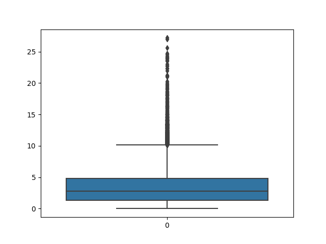
First, let's begin with a boxplot of rebounds. There are ways to do this directly in pandas (nba.boxplot(column=["rebounds"])), but we are going to use the Seaborn library which is a little more powerful and user friendly. It is using the same matplotlib library that pandas is, but it wraps it in nicer functions. The following shows how to produce a boxplot in Seaborn:
sns.boxplot(data=nba.reboundsPerGame)
Depending on your environment, running a command like the one above may bring up the plot automatically for viewing. Or it may just prepare it in the background and wait for you to tell it to show it or save it to a file, etc. This can be done with the matplotlib library that we imported earlier as plt. With this, we can show the current plot or save it to a file:
# Show the current plot
plt.show()

# Save the current plot to a file
plt.savefig("boxplot_reboundsPerGame.png")
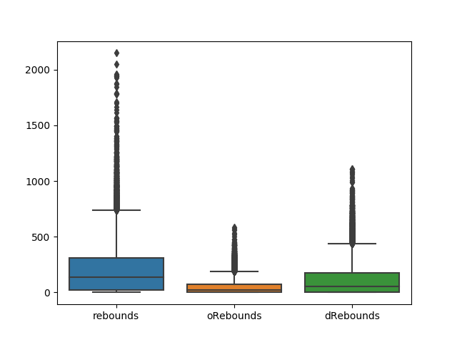
If we want to do a box plot of multiple columns we can also do that. Here are rebounds, offensive rebounds, and defensive rebounds shown together:
sns.boxplot(data=nba[["rebounds", "oRebounds", "dRebounds"]])
Obviously, we would want to clean up the presentation of these graphics with better labels, titles, etc. There are many resources on the internet to help understand the parameters that can be passed to these functions. Please go check them out and see what you can do. A major part of learning to use any kind of libraries, and this is especially true with data science libraries, is developing the skill of finding useful information on the internet.
Rebounds Over Time - Approach 1: FacetGrid
With some basic plotting in place, we are ready to revisit the question of whether rebounding trends have changed over time.
One approach could be to use "facets," and put a whole bunch of small boxplots all next to each other. Seaborn has a facet grid function that makes this fairly easy. It might be too much to have a separate plot for every year from 1930-2010, so let's focus just on the '80s first.
# Get a subset of the data where the year is between 1980 and 1990
eighties = nba[(nba.year >= 1980) & (nba.year < 1990)]
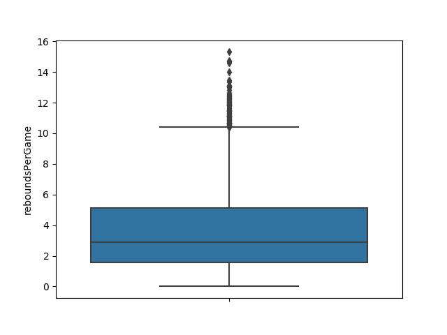
Now let's play around with this to see what we want each facet or mini-plot to look like:
sns.boxplot(eighties["reboundsPerGame"], orient="v")
That seems to look ok, so now we will set up a FacetGrid and map this function for each facet.
grid = sns.FacetGrid(eighties, col="year")
grid.map(sns.boxplot, "reboundsPerGame", orient="v")
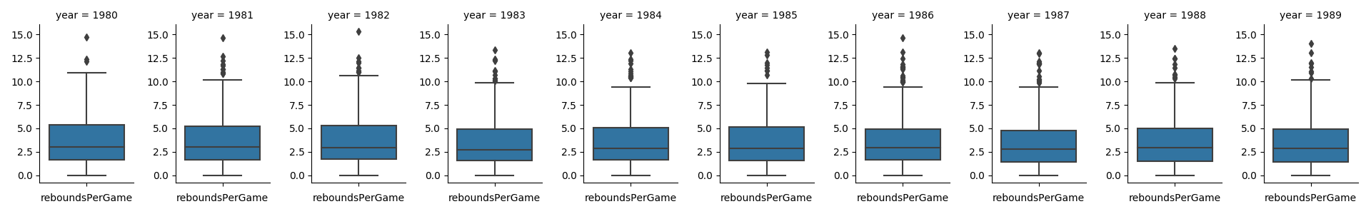
This is nice and contains a lot of information. But it is really hard to see anything related to the trend we want, namely rebounds from the '60s and '70s versus today. So I don't like it. At this point let's abandon the facet grid approach, and instead, perhaps we could just plot a single point per year, like the median number of rebounds for all players for that year, and look for trends in that.
Instructor Tip:
Whoa! Why did we even do these previous steps if we are just going to abandon them?
It turns out that data science is a process of discovery, trial, and error. Sometimes we have an idea, we try it and find out we don't like it, so we have to consider other options. Most tutorials out there (including this one) mostly show the finished product of someone else's discovery process. This is hard, because the important thing for you to learn is actually the process, not the end result.
Rebounds Over Time - Approach 2: Grouping by Year
To plot rebounds per year, we first need to group the statistics by year. When we do so, we need to specify how we want to aggregate the data of that year. In this case, we'll use the median of the reboundsPerGame.
nba_grouped_year = nba[["reboundsPerGame", "year"]].groupby("year").median()
print(nba_grouped_year)
      reboundsPerGame
year
1937         0.000000
1938         0.000000
1939         0.000000
1940         0.000000
1941         0.000000
1942         0.000000
1943         0.000000
1944         0.000000
1945         0.000000
1946         0.000000
1947         0.000000
1948         0.000000
1949         0.000000
1950         0.000000
1951         4.070175
1952         3.417910
1953         3.321078
1954         3.946162
1955         3.893842
1956         4.268657
1957         4.611111
1958         4.586957
1959         4.735294
1960         4.774194
1961         3.733333
1962         4.317319
1963         3.791926
1964         4.076923
1965         4.133333
1966         4.474013
               ...
1982         2.929825
1983         2.689429
1984         2.876894
1985         2.855613
1986         2.904762
1987         2.822117
1988         2.957428
1989         2.857143
1990         2.890244
1991         2.894737
1992         2.805195
1993         2.904283
1994         2.739120
1995         2.685185
1996         2.615385
1997         2.727778
1998         2.728421
1999         2.934768
2000         2.954885
2001         3.098163
2002         3.006494
2003         3.000000
2004         2.813298
2005         2.740533
2006         2.807692
2007         2.823529
2008         2.970149
2009         2.893257
2010         2.856483
2011         3.019434
[75 rows x 1 columns]
Notice that we assigned this to a new variable nba_grouped_year so that we can work with this new version of the dataset that is oriented differently.
In order to plot this data, we need to change the index to be the year now, rather than the id that it was previously. Then we can plot it along with a linear regression line as follows:
nba_grouped_year = nba_grouped_year.reset_index()
sns.regplot(data=nba_grouped_year, x="year", y="reboundsPerGame")
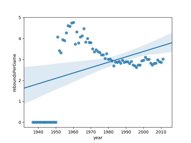
It looks like there are a lot of years where rebounds must not have been tracked (at least in this dataset), so let's remove any years where the median was 0. This time, let's also put a title on the plot.
nba_grouped_year = nba_grouped_year[nba_grouped_year["reboundsPerGame"] > 0]
sns.regplot(data=nba_grouped_year, x="year", y="reboundsPerGame").set_title("Median rebounds per Year")
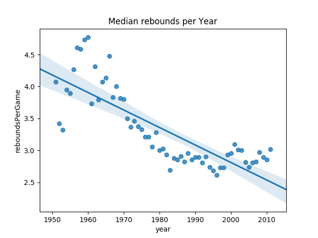
Judging from this plot, it looks like there has certainly been a difference in the rebounding from the '60s versus later years.
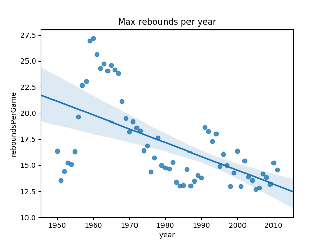
One question we might ask though is, could this be the result of the fact that we just used the median? Maybe there are a lot more players now, and the top rebounders are still just as productive. We could repeat the previous steps, but this time use the max instead of the median.
nba_grouped_year = nba[["reboundsPerGame", "year"]].groupby("year").max()
nba_grouped_year = nba_grouped_year.reset_index()

# Remove the zeros
nba_grouped_year = nba_grouped_year[nba_grouped_year["reboundsPerGame"] > 0]
sns.regplot(data=nba_grouped_year, x="year", y="reboundsPerGame").set_title("Max rebounds per year")
Summarizing in More Complicated ways
From the previous plot, we can still see a similar trend, which makes us feel a little better about our conclusion. However, this summary is still a little bit troubling, because it could be skewed a lot by the top rebounder of that year. Perhaps that rebounder was a major outlier from the rest of the league. Another way to consider this is to find the top 10 rebounders of the year and look at their median.
# Get the top 10 rebounders per year
nba_topRebounders_perYear = nba[["reboundsPerGame", "year"]].groupby("year")["reboundsPerGame"].nlargest(10)

# Get the median of these 10
nba_topRebounders_median_perYear = nba_topRebounders_perYear.groupby("year").median()

# Put year back in as a column
nba_topRebounders_median_perYear = nba_topRebounders_median_perYear.reset_index()

# Again no zeros...
nba_topRebounders_median_perYear_noZeros = nba_topRebounders_median_perYear[nba_topRebounders_median_perYear["reboundsPerGame"] > 0]

# Now plot
sns.regplot(data=nba_topRebounders_median_perYear_noZeros, x="year", y="reboundsPerGame").set_title("Median of Top 10 Rebounders Each Year")
Instructor Tip:
Those are some pretty long variable names! It's up to you what variable names you pick. I often like to choose names that are overly long, so they can be descriptive to a fault. If you are using an editor that autocompletes variable names for you, it's not a problem. But you might choose something a little easier to work with, especially if your editor doesn't autocomplete them.
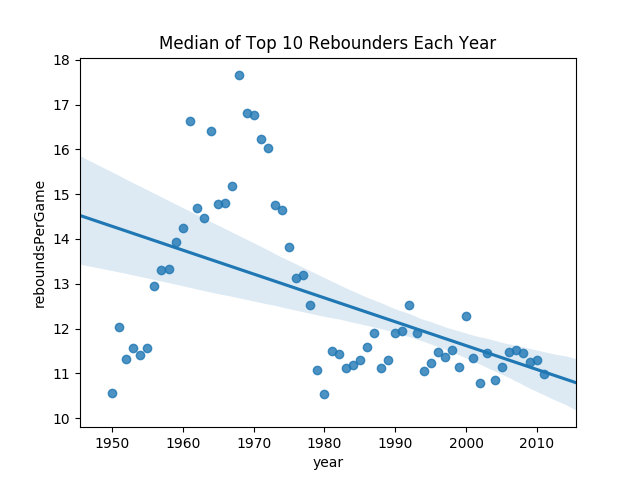
This feels like a more accurate summary of the top rebounders each season, and it seems to help us answer our original question about rebounding trends. From this graphic we can show that the amount of rebounds per game among the top rebounders fluctuates a little, and peaked around 1970.
Concluding Thoughts
This tutorial has walked through the steps of experimenting with rebounds per game, and following questions that might arise in that area.
From this point, we could go on to ask many other questions about this data. What interesting trends can we learn about other statistics? What can we learn about certain players? Are there common characteristics about people from certain eras, hometowns, positions, teams, etc.
Please keep in mind that discovering functions that are available and how to use them is a major discovery process. Following a tutorial like this is really easy, because the work has been done for you of thinking about different options, trying functions that didn't work out well, trying something else, getting errors, looking up solutions on the internet, etc.
This process of discovery, trial, and error takes a lot of work! And this is the real skill that data scientists need. They need to be able to ask questions, like "That's weird, I wonder why ..." and they need to say, "I bet there is a way to put two things on the same plot, I wonder how you do that...". Then you search the internet and figure it out.